2021. 9. 2. 02:37ㆍai/Machine Learning

Tensorflow
-구글에서 만들었다 경쟁사로 페이스북 파이토치가 있다
-파이썬과 sklearn으로만 하기에는 기능이 빈약하고, 어려운면이 있다
- 1.대버전과 2.대버전이 있다 / 두 버전은 호환성이 없다 (외적으로는 많이 안변했으나 내부적으로는 많이 변함)
-도화지에 그래프를 그린다고 생각하면 된다
Tensorflow정의
-open surce software libray이다
-for Numerical computation (수치연산을 위해)
-using dataflow graphs (Node, Edge로 구성된 방향성 있는 graph)
Node : Numerical computation(수치연산, data입출력 담당)
Edge : Node와 Node 사이에 data의 흐르는길
tensor :(동적크기의 다차원 배열: size,차원,길이가 얼만지모른다)연산을 해서 Edge를 통해 다른 Node로 흐르는 data
flow : 흐른다라는 의미
다운로드 - conda install tensorflow==1.15
에러코드 tensorflow-estimator-1.15.1 이걸로 재설치 하시면 깔끔하게 찍혀요
import numpy as np
import pandas as pd
import tensorflow as tf
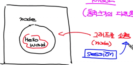
# node 1개 생성해 보아요!
node = tf.constant('Hello World')
# tf.constant() : 상수값이라는 의미이며 값을 넣어준다
# print(node)라고 찍으면 # Tensor("Const:0", shape=(), dtype=string)
# 그래프(노드)를 실행하려면 session이 필요해요!
sess = tf.Session() # 우리가 그린 그래프 실행하기 위한 장치?
print(sess.run(node).decode()) # session을 이용해서 node를 실행
# sess.run() : 세션실행
# .decode() : byte배열을 문자열로 / print했을때 앞에 b가 없어진다

import tensorflow as tf
node1 = tf.constant(10, dtype=tf.float32)
node2 = tf.constant(20, dtype=tf.float32)
node3 = node1 + node2
sess = tf.Session()
print(sess.run(node3)) # 30.0
print(sess.run([node3, node1])) # [30.0, 10.0]

# 두 개의 숫자를 입력받아서 숫자를 더해 출력하는 코드를 작성해 보아요!
import tensorflow as tf
node1 = tf.placeholder(dtype=tf.float32)
node2 = tf.placeholder(dtype=tf.float32)
tf.placeholder() : 빈값이나 추후 값이 들어올거야 즉 변수라고 보면된다
node3 = node1 + node2
sess = tf.Session()
print(sess.run(node3, feed_dict={node1 : 50,
node2 : 100}))
# feed_dict : 먹이를 주는데 dict형태로

# tensorflow의 기본적인 사용법을 배웠으니 이를 이용해서 Multiple Linear Regression을 구현
# 태양광,바람,온도에 따른 오존량 예측에 대한 머신러닝 코드를 작성해 보아요!
# %reset
import numpy as np
import pandas as pd
import tensorflow as tf
import matplotlib.pyplot as plt
from scipy import stats # zscore로 이상치 판별
from sklearn import linear_model # sklearn으로 모델 생성, 학습, 예측하기 위해서 필요!
from sklearn.preprocessing import MinMaxScaler # Normalization을 위해 필요!
# Raw Data Loading
df = pd.read_csv('./data/ozone/ozone.csv', sep=',')
# display(df)
training_data_set = df[['Solar.R', 'Wind', 'Temp', 'Ozone']]
# display(training_data_set.head())
# # 1. 결치값부터 처리해야 해요!
training_data = training_data_set.dropna(how='any')
# display(training_data.shape) # (111, 4)
# # 2. 이상치를 처리해야 해요!
zscore_threshold = 1.8
# # Ozone에 대한 이상치(outlier) 처리
outlier = training_data['Ozone'][np.abs(stats.zscore(training_data['Ozone'])) > zscore_threshold]
training_data = training_data.loc[~(training_data['Ozone'].isin(outlier))]
# display(training_data) # 104 rows × 4 columns
# 3. Normalization(정규화) - Min-Max Normalization
scaler_x = MinMaxScaler() # scaling 작업을 수행하는 객체를 하나 생성
scaler_y = MinMaxScaler()
scaler_x.fit(training_data.iloc[:,:-1].values)
scaler_y.fit(training_data['Ozone'].values.reshape(-1,1))
training_data.iloc[:,:-1] = scaler_x.transform(training_data.iloc[:,:-1].values)
training_data['Ozone'] = scaler_y.transform(training_data['Ozone'].values.reshape(-1,1))
# display(training_data)
#여기까지 저번시간에 했던 전처리
#######################################################
# machine learning code를 작성해 보아요!(Tensorflow)

# Training Data Set
x_data = training_data.iloc[:,:-1].values
t_data = training_data['Ozone'].values.reshape(-1,1)
# 1. 그래프에 입력값을 밀어 넣기 위해 Training Data Set을 받아들이는 node를 생성
# placeholder
X = tf.placeholder(shape=[None,3], dtype=tf.float32)
T = tf.placeholder(shape=[None,1], dtype=tf.float32)
# shape= : 스칼라가 아니고 차원이라면 이를 꼭 명시
# [None,3] : [행 과 열] 이며 안에 None은 np의 [-1]과 같은 의미
# 2. Weight & bias
W = tf.Variable(tf.random.normal([3,1]), name='weight')
b = tf.Variable(tf.random.normal([1]), name='bias')
# tf.random.normal( [행,열], name='이름' ) : np.random.rand랑 같은뜻
# tf.Variable() : tf의변수
# 3. Multiple Linear Regression Model => Hypothesis(가설)
H = tf.matmul(X,W) + b
# tf.matmul() : np.dot()이랑 같은의미 즉 matrix Multiplication (행렬곱)
# 4. loss function
# loss = np.mean(np.power((H-T),2))
loss = tf.reduce_mean(tf.square(H-T))
# tf.square() : np.power() 랑 같은 의미이며 제곱한다라는 뜻
# tf.reduce_mean() : np.mean() 랑 같은 의미이며 평균이라는 뜻
# 5. 학습(Gradient Descent Alorithm을 이용해서(편미분포함) W와 b를 갱신 )
# 1번 편미분해서 W와 b를 갱신하는 역할을 하는 node를 생성(학습)
train = tf.train.GradientDescentOptimizer(learning_rate=1e-4).minimize(loss)
#tf.train.GradientDescentOptimizer (learning_rate= ) :
#train[훈련] Optimizer[최적화] (learnin_rate= 값을 알려줘야한다)
#.minimize() : ()로 줄여줄게
# 6. session & 초기화
sess = tf.Session() # 그래프를 실행시키기 위한 session을 생성
sess.run(tf.global_variables_initializer()) # 초기화
# 반복학습을 진행 -> 학습 Node를 이용해서.
for step in range(300000):
tmp, W_val, b_val, loss_val = sess.run([train, W, b, loss],
feed_dict={X : x_data,
T : t_data})
if step % 30000 == 0:
print('W:{}, b:{}, loss:{}'.format(W_val,b_val,loss_val))
# 학습이 종료되서 W와 b가 최적화 되었어요!
# 7.Prediction (예측)
predict_data = np.array([[180.0,10.0,80.0]]) # Solar.R, Wind, Temp
scaled_predict_data = scaler_x.transform(predict_data) #정규화로 변경
scaled_result = sess.run(H, feed_dict={X:scaled_predict_data}) #예측실행
result = scaler_y.inverse_transform(scaled_result.reshape(-1,1)) #정규화를 원상복구
print(result) # [[40.86704]]
'ai > Machine Learning' 카테고리의 다른 글
| Logistic[논리] Regression 코드 (0) | 2021.09.03 |
|---|---|
| Logistic[논리] Regression (0) | 2021.09.02 |
| Nomalization(정규화),Multiple Linear Regression (다중선형회기) (0) | 2021.09.01 |
| Sklearn(사이키런), 이상치처리 (0) | 2021.08.31 |
| ozone.csv를 python,sklearn으로 LinearRegression 처리 (0) | 2021.08.30 |