2021. 9. 3. 02:22ㆍai/Machine Learning
# Linear Regression으로 Classification문제를 해결할 수 있나요??
# 데이터에 따른 왜곡문제때문에 해결하기 힘들어요!
import numpy as np
from sklearn import linear_model
import matplotlib.pyplot as plt
# Training Data Set
x_data = np.array([1,2,5,8,10]).reshape(-1,1)
t_data = np.array([0,0,0,1,1]).reshape(-1,1)
# sklearn을 이용해서 Linear Regression Model을 생성
model = linear_model.LinearRegression()
# model이 생성되면 학습을 시켜요!
model.fit(x_data, t_data)
# 생성된 Weight와 bias를 출력해보아요!
print('W : {}, b : {}'.format(model.coef_, model.intercept_))
# Prediction을 해 보아요!
print(model.predict([[7]])) # [[0.63265306]]
plt.scatter(x_data.ravel(), t_data.ravel())
plt.plot(x_data.ravel(), x_data.ravel() * model.coef_.ravel() + model.intercept_, color='r')
plt.show()
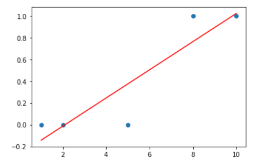
위 코드만 보았을때는 Linear Legration만으로도 가능해보인다 그러나 위 값을 바꾸면 결과가 달라진다
위 코드랑 똑같이 x값 마지막 1개만 바꾸었더니 결과값이 변했다는것을 알수 있다

# sigmoid의 모양부터 살펴보아요!
# Activation Function(활성화 함수)으로 sigmoid함수를 사용할 꺼예요!
import numpy as np
import matplotlib.pyplot as plt
x_data = np.arange(-100,100)
y_data = 1 / ( 1 + np.exp(-1 * x_data) )
# np.exp : e의 지수성을 표현
plt.plot(x_data,y_data)
plt.show()

Logistic[논리] Regression python ver
# 공부시간에 따른 합격여부
# python 구현
import numpy as np
import tensorflow as tf
from sklearn import linear_model
## 수치미분함수
def numerical_derivative(f, x):
delta_x = 1e-4
derivative_x = np.zeros_like(x)
it = np.nditer(x, flags=['multi_index'])
while not it.finished:
idx = it.multi_index
tmp = x[idx]
x[idx] = tmp + delta_x
fx_plus_deltax = f(x)
x[idx] = tmp - delta_x
fx_minus_deltax = f(x)
derivative_x[idx] = (fx_plus_deltax - fx_minus_deltax) / (2 * delta_x)
x[idx] = tmp
it.iternext()
return derivative_x
# Training Data Set
x_data = np.arange(2,21,2).reshape(-1,1) # 공부시간
t_data = np.array([0,0,0,0,0,0,1,1,1,1]).reshape(-1,1) # 12시간은 불합격, 14시간은 합격, 13시간??
# Weight & bias
W = np.random.rand(1,1)
b = np.random.rand(1)
# predict
def logistic_predict(x):
z = np.dot(x,W) + b # linear regression
y = 1 / ( 1 + np.exp(-1 * z) ) # sigmoid 적용, y가 우리의 model
result = 0
if y < 0.5:
result = 0
else:
result = 1
return result, y
# loss function
def loss_func(input_value): # [W의값 ,b의값] 1차원 ndarray로 입력인자를 사용
input_w = input_value[0].reshape(-1,1)
input_b = input_value[1]
z = np.dot(x_data,input_w) + input_b
y = 1 / ( 1 + np.exp(-1 * z) )
delta = 1e-7
return -np.sum(t_data*np.log(y+delta) + (1-t_data)*np.log(1-y+delta))
# np.log : log
# + delta를 넣은 이유는 log 1이 되면 무한값이 되므로 방지용으로 넣었다 1e -8이하로 내려가면 floating error가 날수 있기 때문에 -7로 잡았다
# learning rate 설정
learning_rate = 1e-4
# 반복학습
for step in range(300000):
input_param = np.concatenate((W.ravel(), b.ravel()), axis=0) # [W의값 ,b의값]
result_derivative = learning_rate * numerical_derivative(loss_func, input_param)
W = W - result_derivative[0].reshape(-1,1)
b = b - result_derivative[1]
if step % 30000 == 0:
print('loss : {}'.format(loss_func(input_param)))
# prediction
result = logistic_predict([[13]])
print(result) # (1, array([[0.54454348]]))
# model = linear_model.LinearRegression() # Linear Regression일 경우
model = linear_model.LogisticRegression()
# 학습을 시켜요!
model.fit(x_data, t_data.ravel()) # t_data는 1차원으로 입력해요!
# Prediction
result = model.predict([[13]])
print(result) # [0]
# 그냥 print하면 0 아니면 1 로 떨어진다
result_proba = model.predict_proba([[13]])
print(result_proba) # [[0.50009391 0.49990609]]
model.predict_proba : sklearn의 예측확률을 알려준다
# tensorflow 구현
# placeholder
X = tf.placeholder(shape=[None,1], dtype=tf.float32)
T = tf.placeholder(shape=[None,1], dtype=tf.float32)
# Weight, bias
W = tf.Variable(tf.random.normal([1,1]), name='weight')
b = tf.Variable(tf.random.normal([1]), name='bias')
# hypothesis[ Model ]
logit = tf.matmul(X,W) + b # linear regression model
H = tf.sigmoid(logit) # logistic regression model
# loss function(log loss, cross entropy)
loss = tf.reduce_mean(tf.nn.sigmoid_cross_entropy_with_logits(logits=logit,
labels=T))
tf.nn.sigmoid_cross_entropy_with_logits : tf가 가지는 neural network에 logits을가지고 cross_entropy를 만든다
# train node [w b값 update]
train = tf.train.GradientDescentOptimizer(learning_rate=1e-4).minimize(loss)
# session & 초기화
sess = tf.Session()
sess.run(tf.global_variables_initializer()) # 초기화
# 반복학습
for step in range(300000):
tmp, loss_val = sess.run([train, loss],
feed_dict={X:x_data,
T:t_data})
if step % 30000 == 0:
print('loss : {}'.format(loss_val))
# tensorflow prediction
result = sess.run(H, feed_dict={X:[[13]]})
print(result) # [[0.57887256]] => 합격!!
'ai > Machine Learning' 카테고리의 다른 글
| data 전처리 / 생각해야 할 문제들 (0) | 2021.09.04 |
|---|---|
| 분류 성능 평가 지표(Metric) (0) | 2021.09.03 |
| Logistic[논리] Regression (0) | 2021.09.02 |
| Tensorflow 1.대버전 (0) | 2021.09.02 |
| Nomalization(정규화),Multiple Linear Regression (다중선형회기) (0) | 2021.09.01 |