2021. 9. 29. 01:04ㆍai/Deep Learning
CNN구현 (TF1.15, TF 2.0)
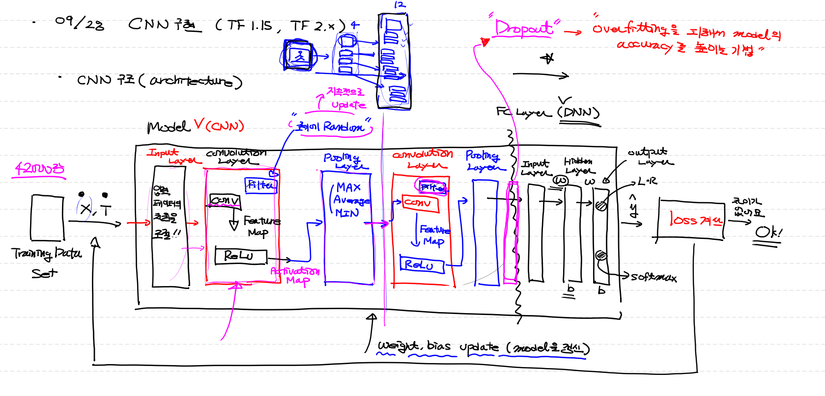
CNN구조 (architecture)
1. Training Data Set (X, T)
2. input layer (입력 data의 차원을 조절 !!)
3. convolution layer
(1) conv ( filter를 이용 [초기값 Random] )
(2) Feature Map 을 Relu 작업
→ activation map
(3) pooling layer (이미지 사이즈 줄이기)
(Max,average,Min 을 이용)
4. 3번작업 반복
(ex) 3번작업에서 4개의 이미지가 나왔다면 4개의 각각 이미지에 대해서 또 4filter 적용 16개 이미지개수가로 늘어난다 /
이미지사이즈는 작아진다)
ㅡㅡㅡㅡㅡㅡㅡㅡㅡㅡㅡㅡㅡㅡㅡㅡㅡㅡㅡㅡㅡ FC Layer (DNN)
5. drop out
6. input layer
7. hidden layer [선택]
8. outpur layer (L ` R, soft max)
9. loss계산 (t,y값) 차이가 별로 없으면 ok
차이가 많이나면 weight, bias update(model갱신)
Drop out : over fitting피해서 model의 accuracy를 높이기 위해 data의 반만 이용
CNN 은 크게 두가지 부분으로 분리해서 생각할 수 있어요!!
1. Feature Extraction (특징 추출) : convolution & pooling layer
2. Classfication (분리) : 학습하고 분류하는 작업
왜 CNN을 사용하나요?
일반적으로 (같은 성능을 내는) CNN(convolution + DNN-적은개수의 hidden layer) 과
DNN(다수의 hidden layer) 을 비교해보면
CNN의 parameter(w,b,filter) 의 개수가 DNN의 parameter의 개수보다 많이 적어요
CNN의 parameter의 수는 DNN의 parameter의 수의 약 20%라 update시간절약 및 성능이 월등히 차이
google Colab 2. 대 버전에서 1.대 버전으로
!pip uninstall tensorflow
!pip install tensorflow==1.15
import tensorflow as tf
print(tf.__version__)
import numpy as np
import pandas as pd
import tensorflow as tf
import matplotlib.pyplot as plt
from sklearn.model_selection import train_test_split
from sklearn.preprocessing import MinMaxScaler
from sklearn.metrics import classification_report
tf.reset_default_graph() # 메모리에 존재하는 tensorflow graph를 reset시키는 작업(1.15버전에서 필요)
# Raw Data Loading
df = pd.read_csv('/content/drive/MyDrive/융복합 프로젝트형 AI 서비스 개발(2021.06)/09월/28일(화요일)/train.csv')
# display(df) # 42000 rows × 785 columns(이미지 42000장)
# MNIST는 2차원으로 된 흑백 이미지를 1차원으로 표현
# 결측치와 이상치는 존재하지 않아요!
# 데이터 확인부터 해 보아요!(matplotplib을 이용해서 그림을 그려보아요! - 10장만 그려보아요!)
# 이미지 데이터만 확보해요!
img_data = df.drop('label', axis=1, inplace=False).values
# subplot을 이용해서 10개만 그림을 그려보아요!
# fig = plt.figure()
# ax = list()
# for i in range(10):
# ax.append(fig.add_subplot(2,5,i+1)) # 2행 5열의 subplot을 만들어서 ax(list)안에 subplot을 저장
# ax[i].imshow(img_data[i].reshape(28,28), cmap='gray')
# plt.tight_layout()
# plt.show()
# Data Preprocessing
# Data Split(Train Data와 Test Data 분리)
train_x_data, test_x_data, train_t_data, test_t_data = \
train_test_split(df.drop('label', axis=1, inplace=False),
df['label'],
test_size=0.3,
stratify=df['label'],
random_state=0)
# MinMaxScaler를 이용한 Normalization(정규화)
scaler = MinMaxScaler()
scaler.fit(train_x_data)
train_x_data_norm = scaler.transform(train_x_data)
test_x_data_norm = scaler.transform(test_x_data)
# Tensorflow 1.15버전을 이용해서 multinomial 처리를 해야 해요!
# => Label에 대한 one-hot encoding처리가 필요!
sess = tf.Session()
train_t_data_onehot = sess.run(tf.one_hot(train_t_data, depth=10))
test_t_data_onehot = sess.run(tf.one_hot(test_t_data, depth=10))
# Tensorflow Graph를 그려보아요! (CNN형태로 그려야 해요!)
# placeholder
X = tf.placeholder(shape=[None,784], dtype=tf.float32)
T = tf.placeholder(shape=[None,10], dtype=tf.float32)
# X 데이터는 convolution 연산을 하기 위한 이미지 데이터로 사용되어야 해요!
# 따라서 X 데이터의 차원을 4차원(이미지개수, 이미지 세로, 이미지 가로, channel)으로 변환
x_img = tf.reshape(X, [-1,28,28,1]) # [None,784] => [-1,28,28,1]
# 첫번째 convolution 연산을 수행할 필터를 생성([필터의 세로, 필터의 가로, 필터의 채널, 필터의 개수])
W1 = tf.Variable(tf.random.normal([3,3,1,32]))
L1 = tf.nn.conv2d(x_img,
W1,
strides=[1,1,1,1],
padding='SAME') # VALID : padding을 사용하지 않아요! 이미지 사이즈가 줄어요!
# SAME : padding을 사용해서 원본과 결과의 크기가 같도록 조절.
# print(L1.shape) # (이미지의 개수, 이미지의 세로, 이미지의 가로, channel) => Feature Map
# (?, 28, 28, 32)
# Relu 연산
L1 = tf.nn.relu(L1)
# pooling layer ( MAX Pooling )
L1 = tf.nn.max_pool(L1,
ksize=[1,2,2,1],
strides=[1,2,2,1],
padding='SAME')
# ksize는 크기 2x2
# stride는 ksize랑 곂치면 안됨으로 ksize값이랑 같이
# print(L1.shape) # (?, 14, 14, 32)
# 두번째 convolution 연산을 수행할 필터를 생성([필터의 세로, 필터의 가로, 필터의 채널, 필터의 개수])
W2 = tf.Variable(tf.random.normal([3,3,32,64]))
L2 = tf.nn.conv2d(L1,
W2,
strides=[1,1,1,1],
padding='SAME') # VALID : padding을 사용하지 않아요! 이미지 사이즈가 줄어요!
# SAME : padding을 사용해서 원본과 결과의 크기가 같도록 조절.
# Relu 연산
L2 = tf.nn.relu(L2)
# pooling layer ( MAX Pooling )
L2 = tf.nn.max_pool(L2,
ksize=[1,2,2,1],
strides=[1,2,2,1],
padding='SAME')
print(L2.shape) # (?, 7, 7, 64)
L2 = tf.reshape(L2, [-1, 7*7*64])
# Feature Extraction
#################################################
# FC Layer를 이용해서(DNN) 학습을 진행.
# Weight & bias
W3 = tf.get_variable('weight3',
shape=[7*7*64,256], # 256 : hidden layer의 node수
initializer=tf.contrib.layers.variance_scaling_initializer()) # He's 초기화
b3 = tf.Variable(tf.random.normal([256]))
_layer3 = tf.nn.relu(tf.matmul(L2,W3) + b3)
layer3 = tf.nn.dropout(_layer3, rate=0.5)
W4 = tf.get_variable('weight4',
shape=[256,10],
initializer=tf.contrib.layers.variance_scaling_initializer()) # He's 초기화
b4 = tf.Variable(tf.random.normal([10]))
# hypothesis
logit = tf.matmul(layer3,W4) + b4
H = tf.nn.softmax(logit)
# loss
loss = tf.reduce_mean(tf.nn.softmax_cross_entropy_with_logits_v2(logits=logit,
labels=T))
# train
train = tf.train.AdamOptimizer(learning_rate=1e-2).minimize(loss)
# session & 초기화
sess.run(tf.global_variables_initializer())
# 반복학습(batch처리를 해야해요! - 메모리 문제때문에)
for step in range(400):
tmp, loss_val = sess.run([train, loss], feed_dict={X:train_x_data_norm,
T:train_t_data_onehot})
if step % 40 == 0:
print('loss : {}'.format(loss_val))
# evaluation
# 우리의 H(hypothesis)는 0~9까지의 확률값을 알려주는 놈이예요!
# H : [0.02, 0.03, ... 0.09, 0.5]
# [0.21, 0.33, ... 0.08, 0.2]
predict = tf.argmax(H,1)
print(classification_report(test_t_data,
sess.run(predict, feed_dict={X:test_x_data_norm})))
import numpy as np
import pandas as pd
import tensorflow as tf
from tensorflow.keras.models import Sequential
from tensorflow.keras.layers import Flatten, Dense, Conv2D
from tensorflow.keras.layers import MaxPooling2D, Dropout
from tensorflow.keras.optimizers import Adam
from sklearn.model_selection import train_test_split
from sklearn.preprocessing import MinMaxScaler
# Raw Data Loading
df = pd.read_csv('/content/drive/MyDrive/융복합 프로젝트형 AI 서비스 개발(2021.06)/09월/28일(화요일)/train.csv')
# display(df) # 42000 rows × 785 columns(이미지 42000장)
# MNIST는 2차원으로 된 흑백 이미지를 1차원으로 표현
# 결측치와 이상치는 존재하지 않아요!
# 이미지 데이터만 확보해요!
img_data = df.drop('label', axis=1, inplace=False).values
# Data Preprocessing
# Data Split(Train Data와 Test Data 분리)
train_x_data, test_x_data, train_t_data, test_t_data = \
train_test_split(df.drop('label', axis=1, inplace=False),
df['label'],
test_size=0.3,
stratify=df['label'],
random_state=0)
# MinMaxScaler를 이용한 Normalization(정규화)
scaler = MinMaxScaler()
scaler.fit(train_x_data)
train_x_data_norm = scaler.transform(train_x_data)
test_x_data_norm = scaler.transform(test_x_data)
# Tensorflow 2.6버전을 이용하기 때문에 Label에 대한 one-hot encoding처리가 필요없어요!
# Keras를 이용한 구현
model = Sequential()
model.add(Conv2D(filters=32,
kernel_size=(3,3),
activation='relu',
input_shape=(28,28,1)))
model.add(MaxPooling2D(pool_size=(2,2)))
model.add(Conv2D(filters=64,
kernel_size=(3,3),
activation='relu'))
model.add(MaxPooling2D(pool_size=(2,2)))
model.add(Flatten())
model.add(Dropout(rate=0.5))
model.add(Dense(units=256,
activation='relu'))
model.add(Dense(units=10,
activation='softmax'))
print(model.summary())
model.compile(optimizer=Adam(learning_rate=1e-3),
loss='sparse_categorical_crossentropy',
metrics=['accuracy'])
history = model.fit(train_x_data_norm.reshape(-1,28,28,1),
train_t_data,
epochs=200,
batch_size=100,
verbose=1,
validation_split=0.3)
model.evaluate(test_x_data_norm.reshape(-1,28,28,1), test_t_data)
'ai > Deep Learning' 카테고리의 다른 글
| cat & dog tf2.0 ver (0) | 2021.09.30 |
|---|---|
| Dog & Cat img → csv (0) | 2021.09.30 |
| CNN 전반적 내용 code (0) | 2021.09.29 |
| convolutional Neral Network (CNN) 합성곱 신경망 (2) | 2021.09.28 |
| 이미지 기본 handling 코드 (CNN기초 ver) (0) | 2021.09.17 |